
by Otto Veltheim, University of Helsinki

Imagine having an unknown system, a “black box”, which outputs identical copies of an unknown quantum state. Suppose our task is to identify the state. There are multiple attributes, i.e. observables describing it, and measuring just one of them makes the state collapse to an eigenstate matching with the measurement outcome. Hence, no further information about the original state can be reliably obtained from the new state. How many copies of the original state and how many measurements do we need then to fully identify the state? This is known as a quantum tomography problem and can be most easily understood via quantum circuits.
We can think of the black box as a quantum circuit which, when given the same input, always outputs the same state. In this setting, any observables to measure can be represented by tensor products of Pauli matrices or their linear combinations. Two different observables cannot, in general, be measured from the same copy of a quantum state, except when they commute, in which case they share an eigenbasis making it possible for the state to collapse to an eigenstate of both observables. Therefore, in order to minimise the required number of measurements, we would like to divide the observables into sets where everything commutes with each other. This commutative property defines a binary relation between the observables, which is symmetric but, unfortunately, not transitive. This makes finding the best ways to group the observables a difficult problem.
The problem can be nicely illustrated with a graph. We can represent the observables as vertices of a graph and draw an edge between two vertices if the corresponding observables do not commute. Then, the problem of trying to find observables which can be measured at the same time reduces to finding sets of vertices in the graph which share no edges. The problem of grouping all the vertices of a graph in this way is a very well-known mathematical problem called graph colouring. In graph colouring, the aim is to assign each vertex of a graph a colour, such that no two vertices sharing an edge are coloured the same. Thus, by colouring the graph of observables, all vertices with the same colour can be measured from the same copy of the state.
Notice that measuring an observable just once does not give us, in general, the correct value of that observable. Each measurement only gives us one eigenvalue of the observable, but we are actually interested in the expectation value, i.e. the average over multiple measurements. We can, of course, use the previously defined groupings and measure each commuting group as many times as is needed for accurate results. Thus, if we need N measurements for each observable in order to achieve the desired accuracy, we just need to multiply the number of groups by N to get the number of state copies that we need. However, we might also be able to do better if we encode this information into the graphs.
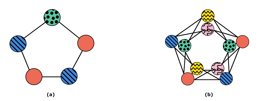
The simplest way to illustrate this is with a cycle graph with five vertices as in Figure 1. Any cycle graph with an odd number of vertices needs at least three colours, as seen in Figure 1a. Suppose, however, that we need to measure each of the observables twice. If we use the measurement scheme in Figure 1a, we will need six copies of the state. If, instead, we include in the graph the information of needing two measurements for each as in Figure 1b, we can find a solution needing only five copies. This generalisation to graph colouring, which introduces weights for the vertices, is known as multicolouring.
The problem of finding an optimal colouring of a graph, i.e. a colouring with the fewest possible colours, is extremely difficult and belongs to the complexity class NP-hard. Thankfully, by giving up on finding the perfect solution, we can usually find some very good solutions even in a time scaling linearly with respect to the number of vertices. With these good-enough solutions, we can end up requiring significantly fewer copies of the state.
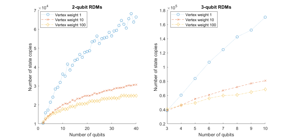
As an example, let us consider trying to determine every k-qubit reduced density matrix of the state of an n-qubit system. This means that we want to measure every tensor product of Pauli matrices, where at least n-k of the tensor product terms are just the identity matrix. In this case, even without assigning weights to the vertices, i.e. if we just use the solution to the regular graph colouring multiple times, the graph colouring scheme can usually find better solutions than many other methods suggested in the literature. However, as shown in Figure 2, by adding weights to the vertices, i.e. allowing multiple colours for each vertex, we can improve the results even further. In fact, it can be proven that without using the weighted graph, the solution would scale as 𝒪(log2𝑛) (as would most other known methods), but using the weighted graph with large enough weights, the solution is expected to scale only as 𝒪(log𝑛).
While many other approaches only focus on solving a specific class of tomography problems, such as the above problem of finding the reduced density matrices, the graph multicolouring method works for any tomography problem. Furthermore, it can be shown that, as long as the tomography problem is defined in terms of observables that can be measured from a single copy of the system, the optimal solution for the multicolouring problem is also the optimal strategy for the measurements.

